Multiclass Confusion matrix made easy for 2×2 and 3×3 matrix

In general, the Confusion Matrix is used to evaluate the performance of a machine learning model. If you are a beginner, when you are trying to decode the confusion matrix, you may end up feeling stuck. In this blog, we aim to decode the confusion matrix for both 2×2 matrix and 3×3 matrix and try to understand both scenarios, including the multiclass confusion matrix.

Whether you’re just starting your career in data science or looking to deepen your knowledge of classification evaluation metrics, this blog is designed in a way that beginners can easily understand by breaking down every terminology in the confusion matrix. We will try to understand everything from scratch by assuming the user is a beginner in the world of data science.

Matrix Structure for 2×2 confusion matrix

Firstly, We will begin the confusion matrix by understanding its structure. To have a clear understanding of matrix structure, i have divided the confusion matrix into two parts. The 1st matrix will have True positive and True negative. In the 2nd matrix false positive and false negative will be displayed.

In the above Matrix, we have 2 dimensions that are Actual values and Predicted Values. The Model predicted to be positive as well as the actual values is also positive then, it is added to the True positive cell. If the Model predicted to be negative as well as the actual values is also negative then, it is added to the True Negative cell.

Accuracy

Accuracy can be defined as the model predicted the correct values, i.e, Total number of True positive and True negative.

Now you can come up with a question, “can we use accuracy also to evaluate the performance of the model ?”

The answer is no because, in case, if the dataset is imbalance, i.e the number of positive class and negative class is not well balanced in the dataset, then it leads to add bias in the dataset. This leads to an increase of Accuracy score.so therefore using only accuracy we cannot conclude the performance of the machine model.

Precision

Precision can be defined as the number of true positives (TP) divided by the sum of true positives and false positives (TP + FP).

Precision tells us how accurate the model is when it predicts a positive outcome. For example, consider a cancer prediction model, precision indicates how correctly the model identifies patients who actually have cancer among all those it predicted as having cancer. Precision does not consider patients who do not have cancer.

Recall

Recall can be defined as the number of true positives (TP) divided by the sum of true positives and false negatives (TP + FN).

Recall tells us how good the model is at identifying all the positive cases. Using the cancer prediction model example, recall indicates how correctly the model identifies all patients who actually have cancer, out of all the patients who do have cancer. Recall does not consider patients who are predicted to have cancer but actually don’t.

Overall, precision focuses on accuracy of positive predictions made by the model and recall focuses on the ability of the model to find all the actual positive cases.

Specificity (True negative rate)

Specificity is also known as True negative rate. Using specificity scores we can identify how well the model can find the negative cases correctly.

For example, in a cancer prediction model, specificity indicates how correctly the model identifies patients who do not have cancer among all those it predicted as not having cancer. Specificity does not consider patients who actually have cancer.

F1 score

F1 Score is the harmonic mean of precision and recall. It provides a single measure of a model’s accuracy that balances both the precision and recall. The F1 score is especially useful when you need to balance precision and recall or when the class distribution is imbalanced.

For example, in a cancer prediction model, the F1 score combines how well the model identifies patients who have cancer (recall) and how accurate it is when it predicts cancer (precision).

Formula for 2×2 confusion Matrix

Accuracy Formula for 2×2 classifier

Accuracy =  \frac{TP + TN}{TP + FP + TN + FN}

Precision Formula for 2×2 classifier

 Precision = \frac{TP}{TP + FP}

Recall Formula for 2×2 classifier

 Recall = \frac{TP}{TP + FN}

F1 score Formula for 2×2 classifier

 F1 = \frac{2 * Precision * Recall }{Precision + Recall}

Calculations of 2×2 confusion Matrix

Let’s take an example to understand the calculation of a 2×2 Matrix. Here we will consider the dataset of cancer patients where positive signifies the presence of cancer and negative signifies absence of cancer. Suppose we have 100 patients and we get the following result from our model:

True Positive (TP) = 50

True Negative (TN) = 25

False Positive (FP) = 15

False Negative (FN) = 10

Now, let’s calculate the evaluation metrics.

Accuracy  =   \frac{TP + TN} {Total} 

 =  \frac{50+25} {100} 

Accuracy = 0.75 or 75%

Precision = \frac{TP}{TP + FP} 

= \frac{50}{50+15}

Precision= 0.77, or 77%

Recall = \frac{TP}{TP+FN}

= \frac{50}{50+10}

Recall = 0.83, or 83%

F1 score = \frac {2 * Precision * Recall}{Precision + Recall}

 = \frac {2 * 0.77 * 0.83 }{0.77 + 0.83}

F1 score = 0.8, or 80%

From this evaluation Matrics, classifier has a accuracy of 75% not bad, but the model requires still more data and training to have a good accuracy score.

Matrix Structure for 3×3 or NxN Matrix

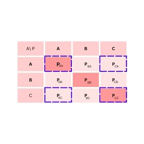
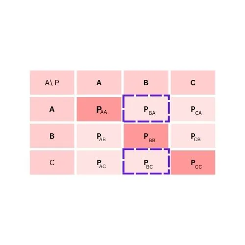
A 3×3 Matrix is used when you have three classes, e.g., ‘A’, ‘B’, and ‘C’. You will have nine cells in the matrix, each signifying different outcomes. For example, if you have predicted value PBA, it means that the model has predicted ‘B’, but the actual value is ‘A’. A 3×3 Matrix will look slightly more complex than a 2×2 Matrix, but the concept remains the same.

P_AA   – this variable correctly predicts the label of A. This acts as a True positive for class A

P_BB –  this variable correctly predicts the label of B. This acts as a True positive for class B

P_CC  – this variable correctly predicts the label of C. This acts as a True positive for class C

P_BA, P_CA – this variable incorrectly predicts labels of A as B  and C.

P_AB, P_CB – this variable incorrectly predicts labels of B as A and C

P_AC, P_BC – this variable incorrecyly predicts labels of C as A and B

Formula for 3×3 Matrix

To calculate True Negative for class A

TN = PBB + PCB + PBC + PCC

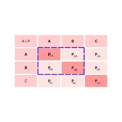
To calculate True Negative for class B

TN = PAA + PCA + PAC + PCC

To calculate True Negative for class C

TN = PAA + PBA + PAB + PBB

To calculate False Positive for class A

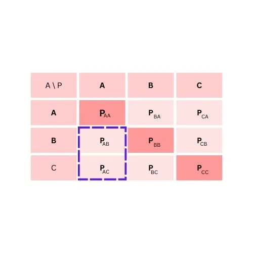
FP = PAB + PAC

To calculate False Positive for class B

FP = PBA + PBC

To calculate False Positive for class C

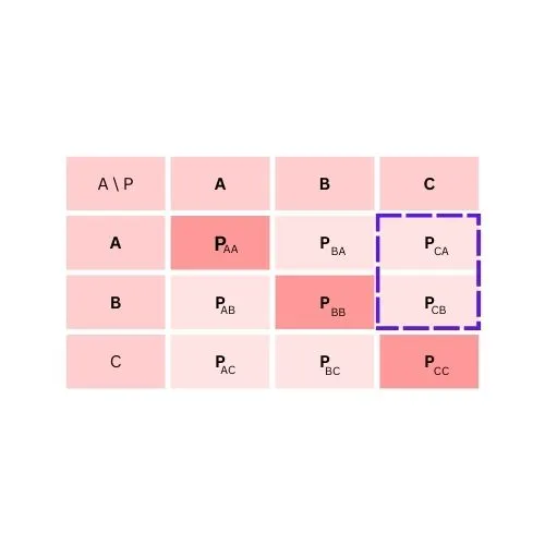
FP = PCA + PCB

To calculate False Negative for class A

FN = PBA + PCA

To calculate False Negative for class B

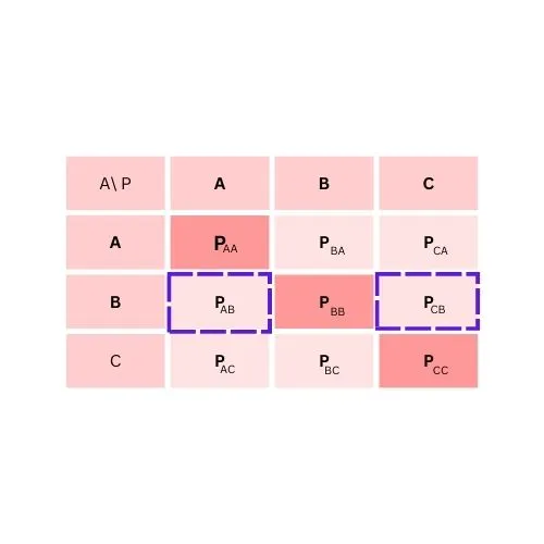
FN = PAB + PCB

To calculate False Negative for class C

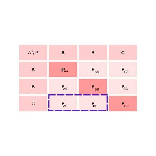
FN = PAC + PBC

Now we can calculate Evaluation metric like Accuracy, precision, specificity and  now easily

Calculations of 3×3 Matrix

Let’s take an example to understand the calculation of a 3×3 Matrix. Here we will consider a dataset of 300 students and we have to predict their grades (A, B, or C). Suppose we get the following results from our model:

PAA = 80,  PBB = 90, PCC = 70,

PAB = 10, PAC = 20, PBA = 10,

PBC = 10, PCA = 10, PCB = 10

Accuracy for class A = (TP + TN) / Total

= (80 + 90 + 70) / 300

= 0.8, or 80%

Accuracy for class B = (TP + TN) / Total

= (80 + 70 + 70) / 300

= 0.73, or 73%

Accuracy for class C = (TP + TN) / Total

= (80 + 90 + 70) / 300

= 0.8, or 80%

You can calculate the other evaluation metrics (Precision, Recall, F1 score) in a similar way.

Precision, Recall, and F1 score are crucial metrics for evaluating the performance of a multi-class classification model. Let’s calculate these metrics for each class (A, B, and C) with the given data.

Precision, Recall, and F1 Score for Class A

True Positives (TP): 80

False Positives (FP) = PBA + PCA

= 10 + 20 = 30

False Negatives (FN) = PAB + PAC

= 10 + 20 = 30

Precision = TP / (TP + FP)

= 80 / (80 + 30)

= 0.73, or 73%

Recall = TP / (TP + FN)

= 80 / (80 + 30)

= 0.73, or 73%

F1 score = \frac{2 * Precision * Recall } {Precision + Recall}

= 2 * 0.73 * 0.73 / (0.73 + 0.73)

= 0.73, or 73%

Interpretation of Multiclass Confusion Matrix

A perfect model will have high values in the diagonal (from top left to bottom right) as these are the correctly predicted values (TP). If your model has high values in other cells, it means your model is making errors.

Type 1 and 2 Error

Type 1 error, also known as a “false positive”, is when we make a positive prediction but the actual value is negative. On the other hand, type 2 error, also known as a “false negative”, is when we make a negative prediction but the actual value is positive.

Examples of Type 1 and Type 2 Errors

To better understand Type 1 and Type 2 errors, let’s look at some practical examples:

Type 1 Error (False Positive):

Imagine you are using a medical test to screen for a particular disease. A Type 1 error would occur if the test indicates that a patient has the disease when, in reality, they do not.

For instance, if a patient is diagnosed with a disease despite being completely healthy, this not only causes unnecessary stress and treatment for the patient but could also lead to wasted medical resources.

Type 2 Error (False Negative):

Conversely, a Type 2 error takes place when the test fails to identify a disease that a patient actually has. For example, if a patient has cancer but the test returns a negative result, the disease may go untreated, potentially leading to serious health consequences for the patient.

This kind of error is particularly critical because it can delay vital treatment and worsen the patient’s prognosis.Understanding these errors is crucial for improving model performance and ensuring reliable predictions in real-world applications.

Conclusion

In conclusion, the Confusion Matrix is an excellent tool to evaluate the performance of your machine learning model. It not only gives you a thorough understanding of how well your model is performing, but also provides insights about where your model is making errors and where you should focus more to improve its performance.

Know about How PCA works, explained step by step in this article